Advanced Usage

Additional inputs to solving routines

Specifiying the Number of Variables Explicitly

num_variables is an optional parameter to eqc_direct.client.EqcClient.solve_integer() and eqc_direct.client.EqcClient.solve_integer(), which defaults to the number of variables inferred from the poly_indices argument, i.e., the largest integer appearing over all the indices. However, a user may specify additional variables that do not appear explicitly in poly_indices. Typically, this is only one additional variable, which creates slack with respect to the sum_constraint, and whose value does not affect the value of the objective function.

As a simple example, if num_variables=3 and sum_constraint=1 so that

x_1 + x_2 + x_3 = 1,

with the objective function given as

f(X) = x_1^2 + x_2^2,

then $x_1 = 0$ $x_{1} = 0$ , $x_2 = 0$ $x_{2} = 0$ , and $x_3 = 1$ $x_{3} = 1$ is a viable solution (giving the ground-state energy $f(X) = 0$ $f (X) = 0$ ). However, if $x_3$ $x_{3}$ were omitted by using the default num_variables=2, then $x_1 = 0$ $x_{1} = 0$ and $x_2 = 0$ $x_{2} = 0$ would not be a viable solution because it would violate the corresponding sum constraint

x_1 + x_2 = 1.

Lastly, due to domain restriction $x_3 \geq 0$ $x_{3} \geq 0$ , $x_3$ $x_{3}$ can only take up so much slack in the problem, so that the subdomain for $x_1$ $x_{1}$ and $x_2$ $x_{2}$ is enlarged but still limited.

Specifiying More than One Sample

The Dirac-3 device is a stochastic solver, and furthermore some problems have multiple solutions that give the same minimum energy. Both of these considerations may indicate the need to run multiple samples that solve the same problem repeatedly on the device. num_samples is an optional parameter to both eqc_direct.client.EqcClient.solve_integer() and eqc_direct.client.EqcClient.solve_integer(), which defaults to one sample. Pass an integer greater than one to run multiple samples more efficiently as a “batch” in a single job. Additionally, running multiple samples in a single batch can save some time in pre-processing since it is only necessary to apply the formatting to submit the problem to the device a single time.

Device Configurations

Dirac-3 allows users to control the optimization process using the relaxation schedule parameter. This parameter controls the time allocated for the system to evolve and converge towards the ground state and is available for both solver types.

Schedules 1, 2, 3, and 4 correspond to different time settings, with higher schedule numbers indicating slower system evolution. Consequently, this leads to a higher probability of obtaining favorable results. Additionally, there are two different device settings that can modify each relaxation schedule:

mean_photon_number: Sets the average number of photons present in a given quantum state. Allowed range: [0.0000667, 0.0066666].
quantum_fluctuation_coefficient: specifies the number of photons ( $N$ $N$ ) for each feedback loop which controls the shot noise. The number of photons is inversely related (e.g. increasing number of photons decreases noise; fewer photons increases noise) to the shot noise with the following equation:

$\delta x \propto \frac{1}{\sqrt{N}}$

Allows integer values from [0,100].

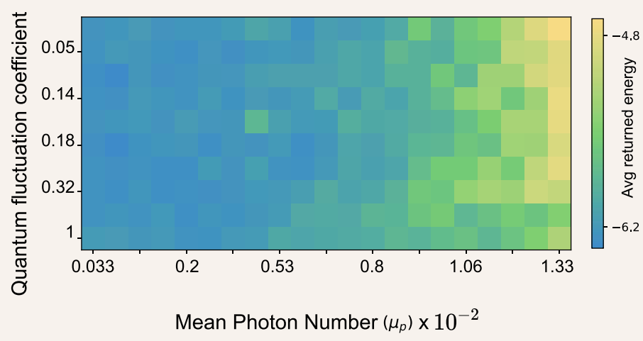
If not specified, the system defaults for each schedule will be applied. These parameters are still an active area of research, so manipulation from standard schedules is considered experimental. Below is an example of a parameter sweep taken for LABS 10:

prop_optimal_labs_10 — A sweep of values for `mean_photon_number` and `quantum fluctuation coefficient` on problem QPLIB0018 from the library of quadratic programming instances (QPLIB) (Furini et al, 2018)

An example using relaxation schedule with tuned parameters

Find the minimium of:

f(X) = (x_1 - 1)^2 + (x_2 - 1.375)^2

where $x_1$ $x_{1}$ and $x_2$ $x_{2}$ are both in $\{0, 0.5, 1, 1.5, 2, \ldots\}$ ${0, 0.5, 1, 1.5, 2, \dots}$ , i.e, minimizing over a non-integral lattice in the positive quadrant.

By inspection, we can see that, without any domain restriction, $f(X)$ $f (X)$ has a unique global minimum of zero at $x_1 = 1$ $x_{1} = 1$ and $x_2 = 1.375$ $x_{2} = 1.375$ . However, that solution is not on the lattice domain, so one expects the optimal feasible solution to be $x_1 = 1$ $x_{1} = 1$ and $x_2 = 1.5$ $x_{2} = 1.5$ with $f(X) = 0.015625$ $f (X) = 0.015625$ .

We now verify this using using Dirac-3. First, expand $f(X)$ $f (X)$ as a polynomial:

f(X) = x_1^2 - 2 x_1 + 1^2 + x_2^2 - 2.75 x_2 + 1.375^2.

Dropping the constant terms, which do not affect the minimization problem and are not supported by Dirac-3, gives:

f(X)' = x_1^2 - 2 x_1 + x_2^2 - 2.75 x_2.

This minimization problem does not appear to be particularly hard, so we will start with relaxation_schedule=1. We need to choose a sum_constraint, num_variables, and solution_precision to search a sufficiently large portion of the domain lattice spaced at 0.5 in each variable. This can be difficult in larger dimensional problems where one has less insight as to where the optimal solution may lie. Furthermore, the sum constraint means that the domain searched forms a non-rectangular simplex. To this end, we take num_variables=3, sum_constraint=3, and solution_precision=0.5, so that the constrained domain is large enough to encompass the region where we suspect the optimal solution to lie. Lastly, we set num_samples=5 to examine repeatability.

from pprint import pprint
import numpy np
from eqc_direct.client import EqcClient
# MUST FILL IN THE VALUES IN THIS FROM YOUR NETWORKING SETUP FOR THE DEVICE
client = EqcClient(ip_address="<YOUR DEVICE IP ADDRESS>", port="<YOUR DEVICE PORT>")
poly_indices = np.array([[0, 1], [0, 2], [1, 1], [2, 2]], dtype=np.uint32)
poly_coefficients = np.array([-2.0, -2.75, 1.0, 1.0], dtype=np.float32)
# use lock to prevent other users from taking exclusive access to the device
lock_id, start_ts, end_ts = client.wait_for_lock()
print(f"Waited for lock: {(end_ts - start_ts) / 1e9} s for lock_id={lock_id}.")
try:
    result = client.solve_sum_constrained(
        lock_id=lock_id,
        poly_indices=poly_indices,
        poly_coefficients=poly_coefficients,
        num_variables=3,
        sum_constraint=3,
        solution_precision=0.5,
        mean_photon_number=0.00333,
        quantum_fluctuation_coefficient=4,
        num_samples=5,
    )
    print("Total execution time (s):",
          np.array(result["preprocessing_time"])+np.array(result["postprocessing_time"])+np.array(result["runtime"]))
    pprint(result)
finally:
    # release lock when finished using the device
    lock_release_out = client.release_lock(lock_id=lock_id)
    print(f"Lock release returned {lock_release_out}")

Additional Resources

To learn more about the theory and function of the device please use the followign resources:

Dirac-3 User Guide
Entropy Computing: A Paradigm for Optimization in an Open Quantum System (Nguyen et al, 2025)

Troubleshooting and Support

If you encounter any issues or errors that are not covered in this manual or the user guide for the device and require additional assistance contact our customer support at https://quantumcomputinginc.ladesk.com.